This is from a research project with Oliver Priebe related to Dr Ted Chinburg’s ‘Entropy and the Mathematics of Evolution’ seminar.

Project Summary

Our visual system is a highly complex network of biological mechanisms shaped by millions of years of evolution. For simplicity, we will consider the eyes as a grid of pixels that responds to the electromagnetic spectra that enter the eye and are focused onto the retina.

Incredibly, this machinery gives us the ability to sense ~30 frames a second of color imagery, each the equivalent of tens of millions of pixels, which together equates to about 1 Gigabyte/second of visual data. To put this into perspective, an entire 2 hour movie in 4k requires about 100GB of data.

This immense amount of data leads us into the main questions of our project: How are we able to process all of this information to form our perception of reality? How can we simulate scenes to trick the brain into ‘seeing’ spaces that do not exist? And finally, how do we possibly store all of this information in our memory?

Here we attempt not to answer these questions in full, but rather to take the reader on a journey through the mathematics of vision and learn some new techniques along the way.

Part I: The Rendering Problem

1. Introduction

1.1 Data of Color Perception

In graphics, light is understood as a binning of wavelengths based on what the human eye can actually perceive. In terms of discrepancy between colors, when tested against different hue variations, studies show that individuals begin perceiving small differences between color choices at the 7\text{-bit} level, so to maintain continuity, 8\text{-bit} is conventionally used (12\text{-bit} for professional photo quality, 24\text{-bit} for the extremists and graphic designers who want the 4 million color choices).

Physical devices can only produce a subset of these combinations of the complete color space defined by CIE (Commission International de l’Eclairage) due to limitations of machinery, lighting, and ink quality [Figure 1]. These conventional subspaces, CMYK, sRGB, and Hexachrome, are common labelings found on most ink and screen-based devices. All these colors can be boiled down to a linear combination of red, green, and blue continuous quantities; however, in these limiting spectra defined by the visual CIE space actually available and binned for output, advanced rendering engines are able to still recreate the full visual spectrum by discretizing the space with the bit quantities previously mentioned.

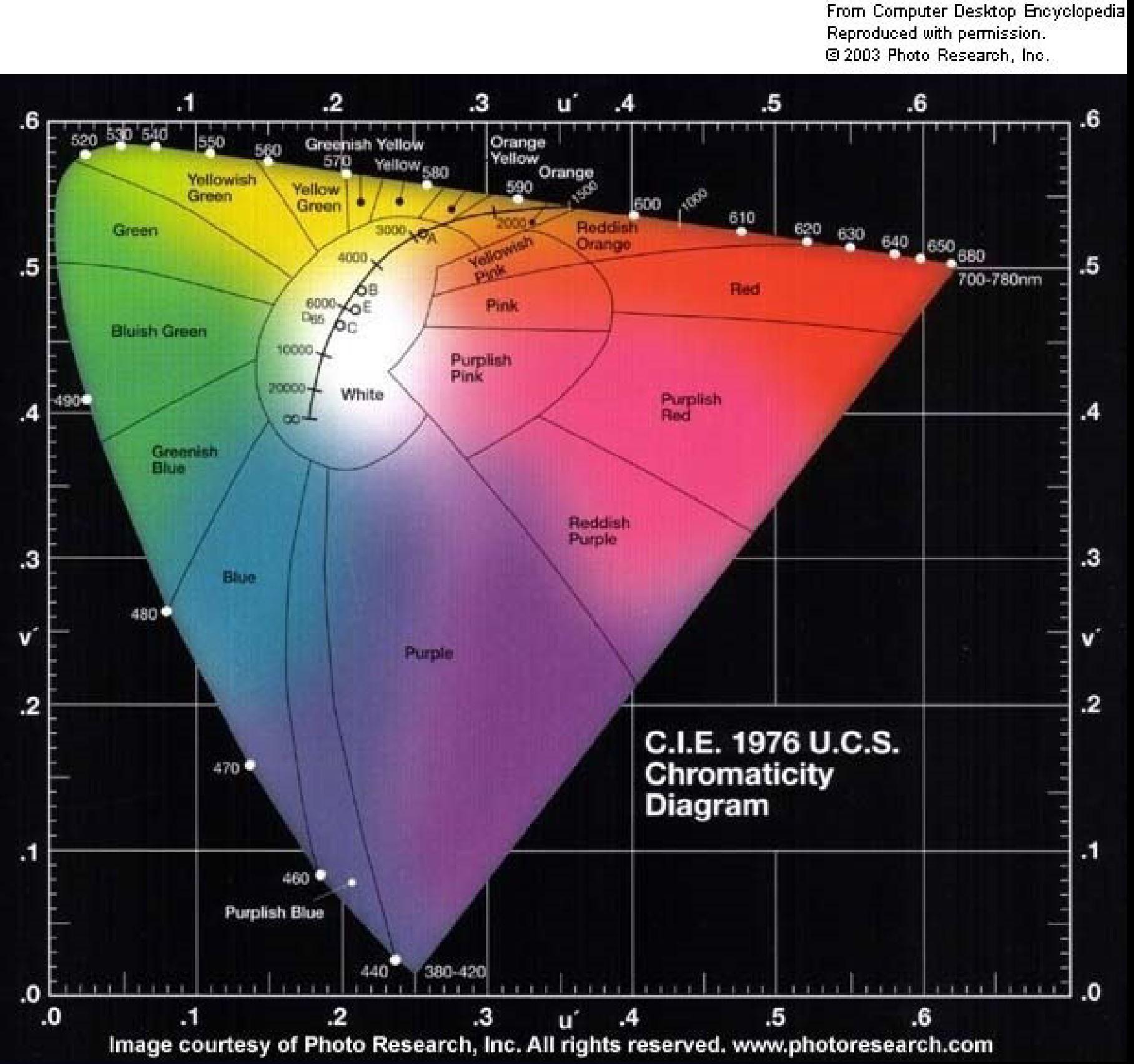
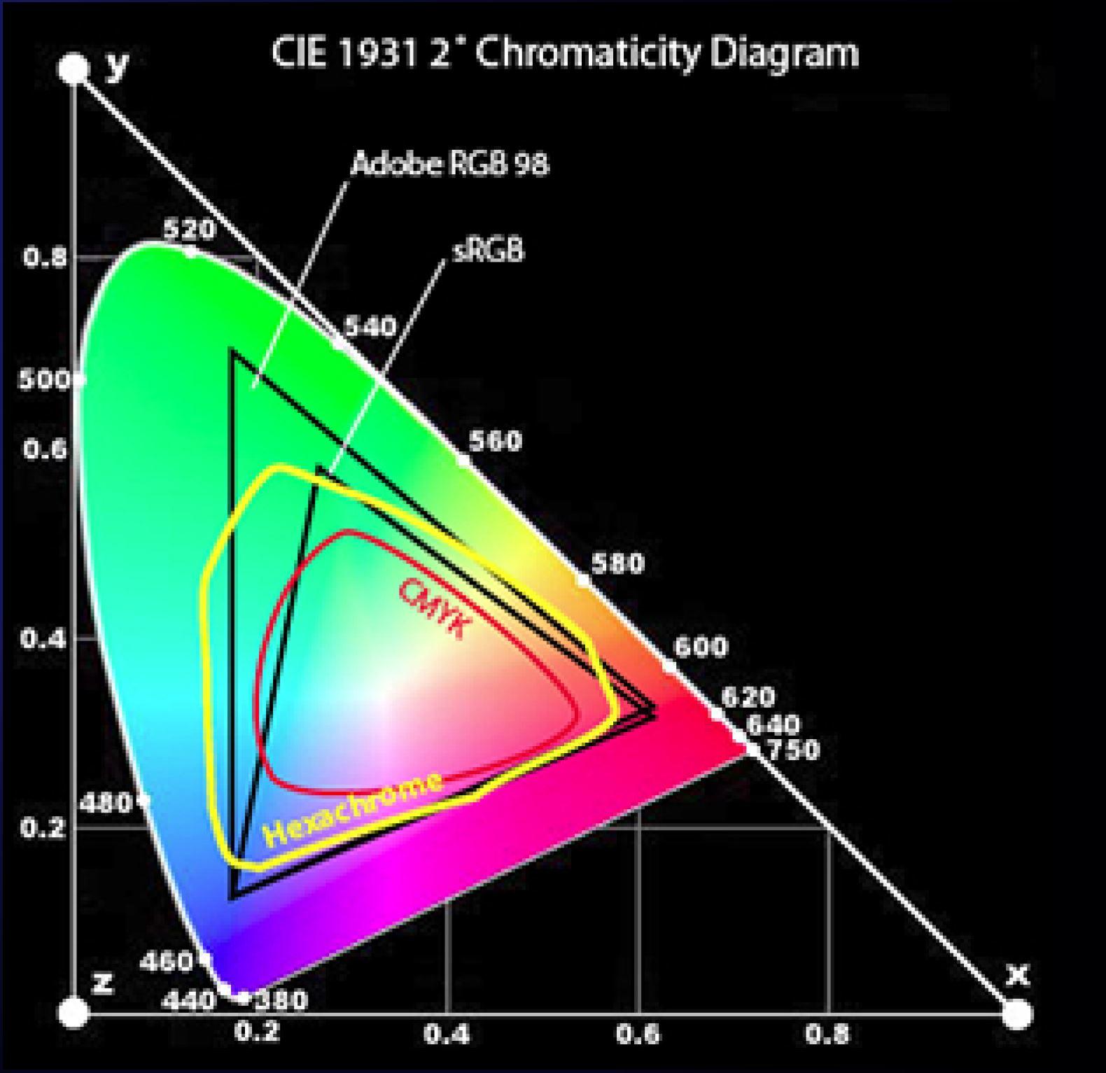
Figure 1: Left - The CIE Chromaticity Diagram of general spectral colors viewable by the human eye. Right - A variation of the CIE Chromaticity Diagram sectioned with conventional device subspaces. (photoresearch.com)

In rendering, these ideas of coloring for pixels gets quantified computationally by macroscopic physics on the scale of general scene dynamics and geometry and by microscopic physics in terms of materials used and surface properties. Additionally, sampling becomes essential to rendering as it is the basis for how color and ray bouncing has been able to closely emulate the pseudorandom volume covering aspect of light radiance.

1.2 Some Rendering Definitions

All of computer graphics is just layering upon layering of matrix manipulations and linear algebra techniques to alter numbers for a color output. None of it is visually real and none of the geometry is actually tangible, making transformations, space conversions, and vector manipulations incredibly important for the math to create the proper output. Here are some beginning definitions to get started; they are common terms used in linear algebra, yet have their definitions specified a bit more to be understood for their uses in computer graphics. These definitions will be used in further detailed explanations so they are added here as reference.

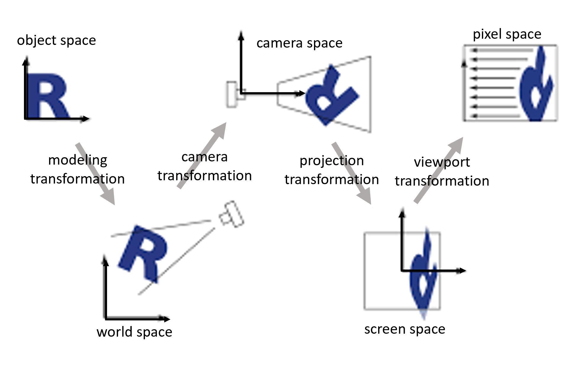
Figure 2: The different transformation spaces and how they are related to one another.

Camera/View Space: 3D space, the scene from the camera’s point of view.

Screen Space: 2D space that fills a square section covering the screen that is normalized such that it ranges from (-1, -1) to (1, 1).

Pixel Space: 2D space that is a version of Screen Space just scaled so that its corners are now proper for the screen at (0, 0) to (\text{width}, \text{height}).

World Space: The conventional space of all 3D points in the scene at their proper locations.

Object Space: The loaded-in version of the geometry as it is represented in its file. For example: the convention of object space for a sphere is centered at [0, 0, 0]^T with no rotation and a radius of 1.

Camera/View Matrix: The scene in terms of the camera or eye’s point of view. Since it’s impossible to move the camera itself (since it’s not physical), the matrix actually does a reverse of the view transformation moving the scene around the camera instead to mimic the ‘viewing’ effect (like geocentric versus heliocentric).

Projection Matrix: It’s a 4 \times 4 matrix that converts 3D View Space to Screen Space. That is, it converts all geometry points that are vectors [x, y, z]^T by working with z as the depth coordinate that the near and far plane divides by distance. To do this calculation, we actually begin with any 4-vector of the form [x, y, z, w]^T because the w coordinate allows for 3D space transformation matrix calculations. Ultimately the projection matrix manipulation ends up setting z = w, creating [x, y, z, z]^T which properly creates a depth space for the near clip and far clip planes of the frustum. Then dividing by the z-value creates a homogenized vector in screen space and creates the perspective effect of a vanishing point at the center of the screen.

Model Matrix: Not all geometry in the final 3D scene is of the same dimensions as it was loaded. The model matrix acts as a way to position, scale, and rotate any object to its desired setup. Converts from a geometry’s Object Space to its World Space representation.

Normal Vectors: [x, y, z, 0]^T — The 4th coordinate is 0 to prevent any translational transformation matrices from skewing the vector. Additionally, the vector is unit length.

Positional Vectors: [x, y, z, 1]^T — The 4th coordinate is 1 to allow for homogenized transformation matrix multiplications.

Ray: A set of two vectors that act as an origin [x, y, z, 1]^T and a normalized direction [x, y, z, 0]^T. An intersection found along this ray is at distance t from the origin such that its location on the ray is of the form:

r(t) = \text{ray}_{\text{origin}} + t \cdot \text{ray}_{\text{direction}}

Ray-Intersection: The World Space location on a piece of geometry of a ray hitting it. To actually solve for this piece of information, the ray is transformed from World Space to the geometry’s Object Space for ease of intersection calculation (for example: it’s easier to find the intersection of an unskewed unit sphere at [0, 0, 0]^T than it is to find one of a rotated oval at an arbitrary location). The values returned for this intersection (\text{isx}) include the t value based on the World Space version of the distances between the ray’s origin and the point found, the surface normal (and sometimes the associated tangent and bitangent vectors), and the materials of this surface. So it goes \text{Model}^{-1} \cdot \text{ray}_{\text{origin}} and \text{Model}^{-1} \cdot \text{ray}_{\text{direction}} to convert to find the intersection in Object Space; then to convert back out to World Space, it goes \text{Model} \cdot \text{isx}_{\text{position}} and (\text{Model}^{-1})^T \cdot \text{isx}_{\text{normal}}. The (\text{Model}^{-1})^T is to remove the scale aspect of the transform that would ruin the perpendicularity quality of the surface-normal.

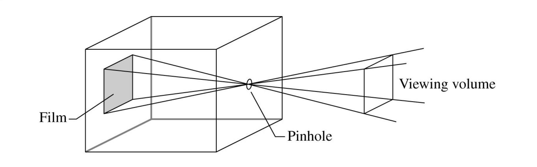
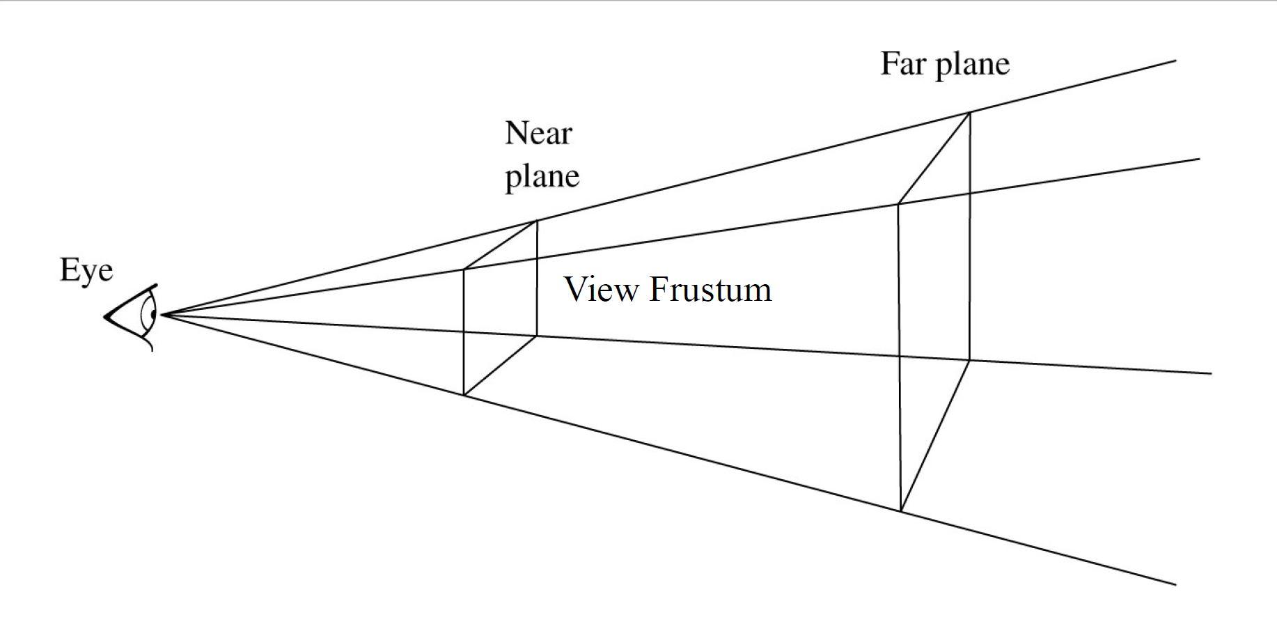
Figure 3: Left - A conventional pinhole camera. Right - The frustum based camera that recreates the pinhole effect just with the eye acting as the capture space. The geometry is homogenized between the near and far planes of the scene such that anything closer or farther from those quantities is considered either too close or too far to be viewed in the scene.

Camera: Most rendering techniques follow a camera and scene model in which the viewing screen acts as the camera itself; however, instead of following the actual camera model (which is based on the pinhole idea), the mathematics of the interaction is abstracted into a frustum approach [Figure 3]. Certain techniques involve a force-able way of slapping the items in the scene onto the screen such as through rasterization of the points (more common in games due to its speed) which uses \text{Projection} \cdot \text{View} \cdot \text{Model} \cdot [x, y, z, 1]^T; however, most ray-based techniques use the camera as a starting location for samples. This idea follows that each pixel acts as a mini camera itself by shooting a ray (or rays) directly into the scene to propagate as if it is following the reverse of a bounce of light on its way from a source to the camera’s pixel. This propagation idea will be further detailed in the Rendering and Sampling section.

1.3 Light and the Light Transport Equation

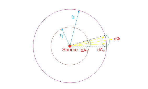
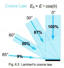
Figure 4: Lambert’s law demonstrated in the 3-dimensional and the 2-dimensional sense. For a source with the same initial intensity, covering a larger area due to angle or distance decreases the intensity per unit area. That is, a light bouncing at a steeper angle will have a softer surface than a light bouncing directly at a surface with perpendicularity. This can also be thought of as \omega_i \cdot n; the dot product of the incident light and the surface normal.

The physical quantity of light can be thought of as an intensity or power per unit area (e.g., for a spherical source, I = \frac{P}{\pi r^2}). When quantizing this value in terms of a discrete area on the surface of a representative sphere, the incident radiance for that differential location is:

dE = \frac{\Phi \cos\theta}{4\pi r^2}

which includes the 1/r^2 power fall-off and Lambert’s cosine law of illumination [Figure 4].

In graphics terms, this color and intensity of a light source is quantified as a float-based RGB vector with each value ranging from [0, 1]. Additionally, the light quantities are additive; that is, the illumination of several lights can be computed separately and summed together for the final total. The scaling to reach the same range [0, 1] all depends on the influence of Lambert’s law, a statistical weighting of each incoming ray sample’s influence.

To continue, the Light Transport Equation (LTE) can be thought of as depending on its incoming (\omega_i) and outgoing (\omega_o) rays of light at each iterative bouncing step of the tracing system (aspects of bouncing discussed in 2.1) [Figure 5]. We use these directions to propagate the color of the light as it bounces throughout the scene. To start we sum the radiance emitted by an object at a specific point (L_e(p, \omega_o)), plus the sum of all the reflected light at that point based on its material properties with f(p, \omega_o, \omega_i) corresponding to the surface’s probabilistically sampled color value based on its material types, L_i(p, \omega_i) corresponding to the recursive summing of future bounces along the \omega_i direction, and |\cos\theta_i| for Lambert’s law at that differential surface area (d\omega_i) of the entire spherical sampling volume. That is, the total incident light at a point p is the following formula:

L_o(p, \omega_o) = L_e(p, \omega_o) + \int_{S^2} f(p, \omega_o, \omega_i) \cdot L_i(p, \omega_i) \cdot |\cos\theta_i| \, d\omega_i

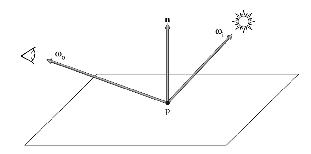
Figure 5: Direction of light bounce and labeling. \omega_i is the incoming direction bounced from the light, \omega_o is the outgoing direction due to the intersection, and n is the normal at that intersection. When propagating from one intersection to the next following the direction from eye to bouncing throughout the scene, \omega_o becomes \omega_i at the next iteration; however, all calculations need to be done with \omega_o and \omega_i pointing out of their concerned intersection, so the recursive \omega_o is commonly flipped during calculations to point out of the intersection as depicted.

2. Rendering and Sampling

2.1 Introduction to Rendering Techniques

So now we have an understanding of the camera, the scene, and ray propagation, but how do we actually use this for filling in pixels on a screen? Rasterization, Raytracing, Pathtracing, and Photon Mapping are common ways to do just that. Rasterization is commonly found in most ‘pre-made’ rendering pipelines you’ll find on your computer such as DirectX, OpenGL, Swift, etc. This pipeline was one of the original styles of converting features to pixel space for three-dimensional visualizations. As explained in 1.2, it doesn’t involve sampling since it is just matrix space transformations from World Space to Pixel Space. Raytracing involves a propagation of a ray bouncing from the camera into the scene for each pixel, bouncing based on a probabilistic material property at each surface, and resolving one pixel through that one recursive aspect [Figure 7].

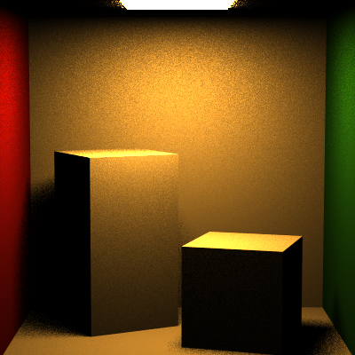
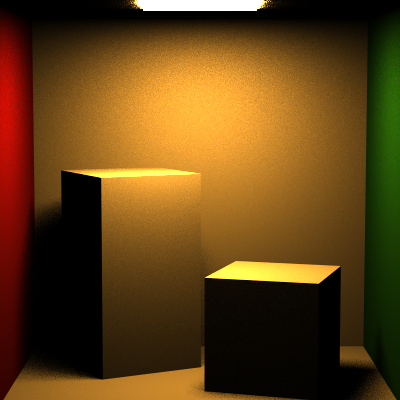
Figure 6: Left - A simple scene render of 512 \times 512 pixels at 5 spp, ~5min render time. Right - The same scene at 10 spp, ~7min render time. Notice the larger amount of noisiness on the left (especially in the shadowy area), yet there is still noise in both scenes.

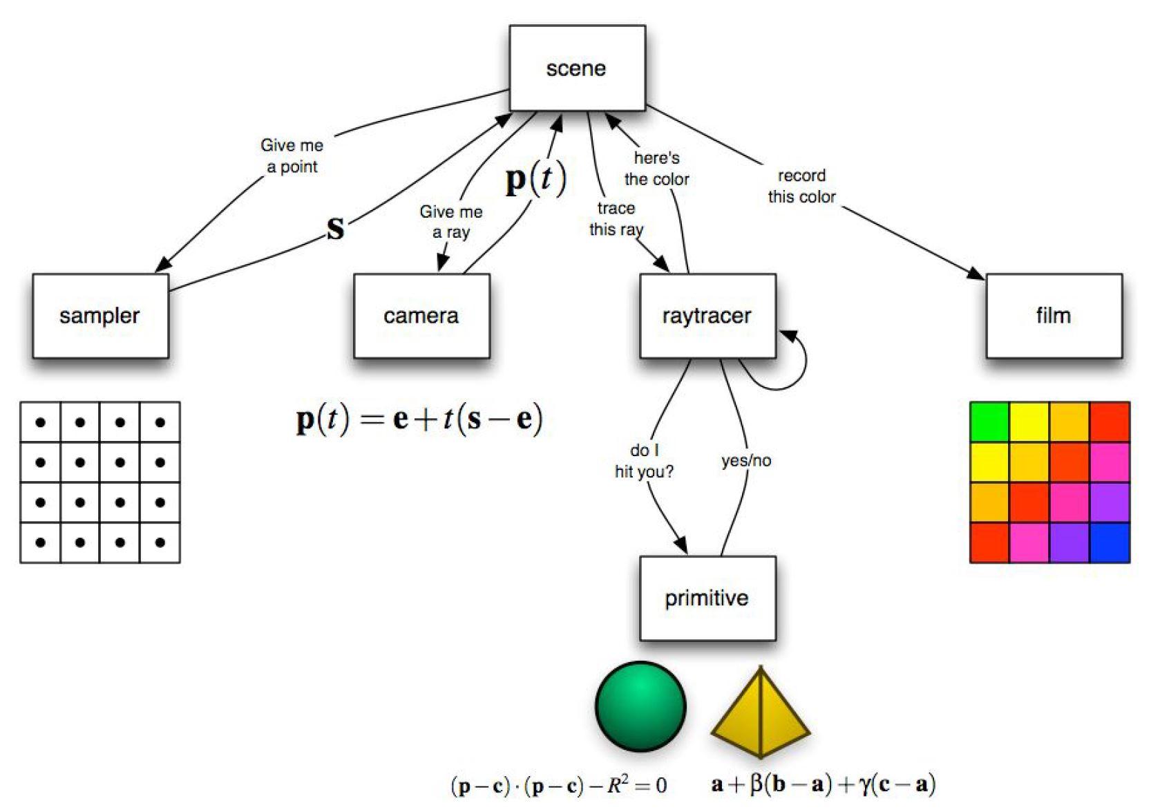
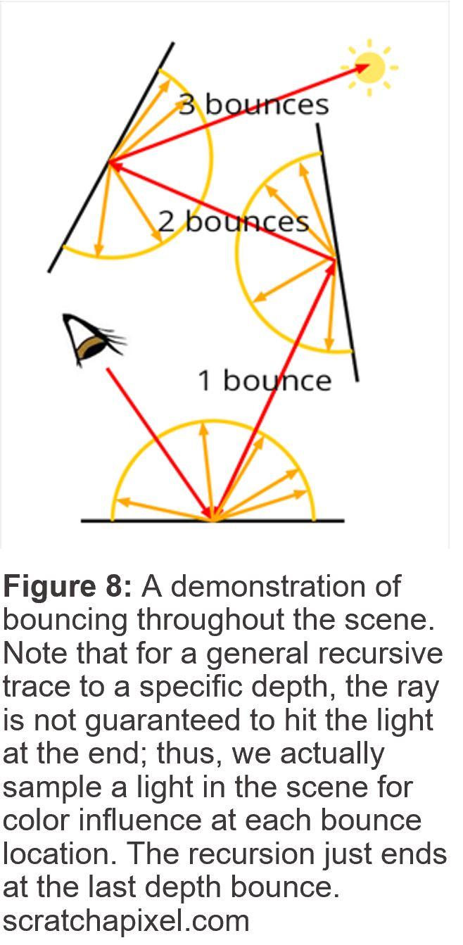
Figure 7: Left - A breakdown of the steps of a raytracer for visual understanding. Right - A demonstration of bouncing throughout the scene. Note that for a general recursive trace to a specific depth, the ray is not guaranteed to hit the light at the end; thus, we actually sample a light in the scene for color influence at each bounce location. The recursion just ends at the last depth bounce. (scratchapixel.com)

Pathtracing takes Raytracing a step further and for each pixel, it samples multiple starting locations and at each intersection location it finds in the scene, samples bounce probabilistically as well. Thus, if the setup starts at 5 spp (samples per pixel), a 512 \times 512 pixel image on a scene of just a cube with a test depth of 3 for number of recursive bounces will have at most 3,932,160 total bounce locations in the scene where calculations are required [Figure 6]. Such a small number of spp does not converge onto a nicely rendered scene, yet properly implemented with all bouncing aspects will still take about 5 minutes to run by itself. This is pretty slow considering the small size of the image and simplicity of the scene.

Recent screens at 1080p (1080 \times 1920 resolution) and 4K (3840 \times 2160 resolution) have about 31,104,000 (~39 min) and 124,416,000 (~158 min) respectively on that scene with those same spp and bouncing credentials. A more detailed scene would have a longer runtime at each bounce location due to the complexity of searching for intersections in the scene leading to even longer runtimes. This is way too long for industry standard. Searching techniques help speed up the runtime per bounce; however, there are still issues in terms of the final output due to such a low initial sample count. Thus, initial sampling techniques at each pixel become incredibly vital for synthesizing renders in a timely manner by allowing for reduced sample counts without losing visual coherency of the scene for the human eye.

2.2 Monte Carlo Sampling

For actual rendering techniques there are a few different cases in which sampling occurs. To start, how do we actually sample the pixels in the first place before we shoot a ray into the scene? With just one spp, it can be simplified down to either an exact location (for example: center or corner) or a randomly applied location specifically for that pixel; however what happens if there are multiple samples? To ensure proper coverage, stratified grid sampling is used. That is, instead of just randomly sampling the pixel as a whole, grid sampling is used, but with a random jittered offset for that sample at that grid location in the pixel [Figure 8].

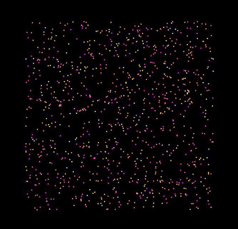
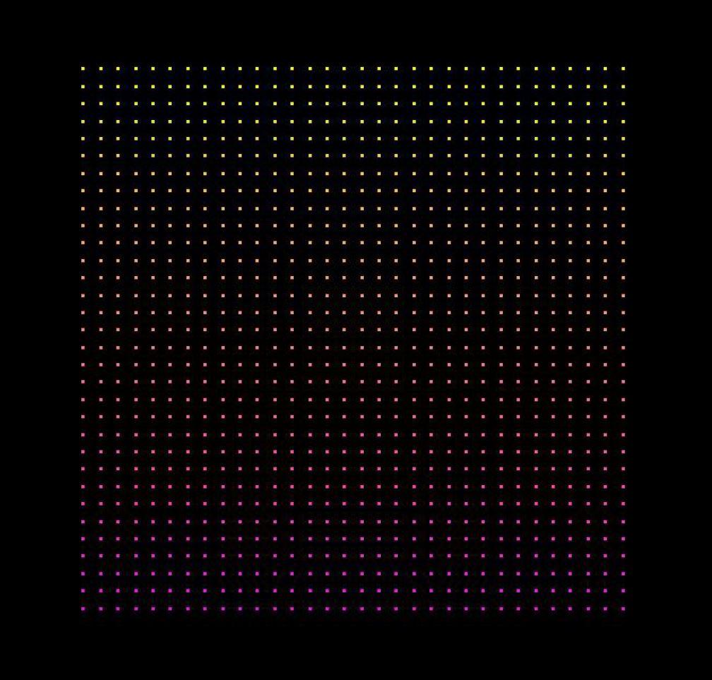
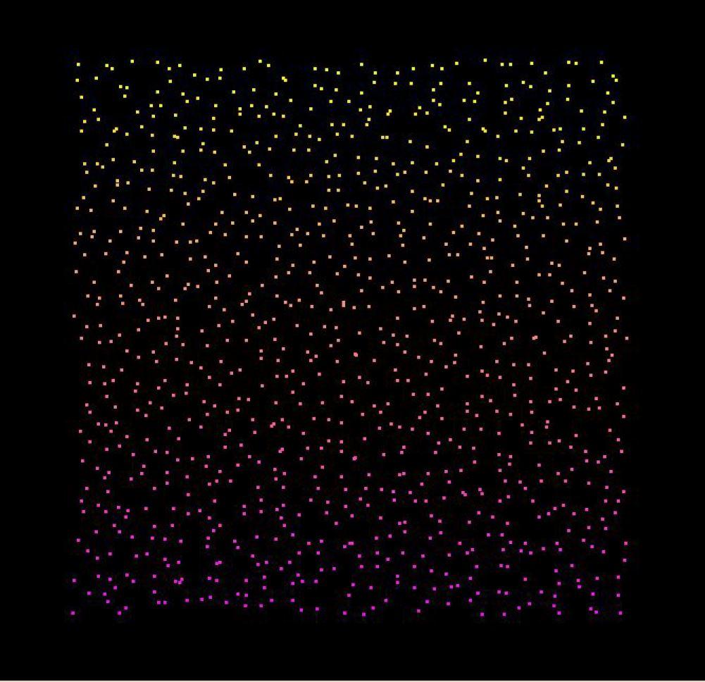
Figure 8: Comparison of pixel sampling techniques. Left - Purely random sampling of a pixel. Middle - Purely gridded sampling of a pixel. Right - Stratified sampling of a pixel (notice the more even distribution yet it still maintains pseudo-randomness).

Then, at each intersection location in the scene we also have to sample where we’ll be bouncing next based on certain material properties. Monte-Carlo integration as a basis is fundamental for allowing this sampling to work. Looking back at the LTE, the idea behind its discretization mentioned before, is to take random samples along the integral over the surface S^2 of possible bounces and average out the results. Note that this maintains that the outcome depends on the samples taken; with a few number of samples there’s a large discrepancy between the actual results and real-life, and by increasing the overall sample count, this error on the average can be decreased (though it increases the runtime drastically).

In terms of the mathematical derivation, it follows that the expected value of light for a sample at an intersection location depends on the discretized weighting and averaging of each of the possible samples:

L_o(p, \omega_o) = L_e(p, \omega_o) + \int_{S^2} f(p, \omega_o, \omega_i) \cdot L_i(p, \omega_i) \cdot |\cos\theta_i| \, d\omega_i

L_o(p, \omega_o) = L_e(p, \omega_o) + \int_0^{2\pi} \int_0^{\pi/2} f(p, \omega_o, \omega_i) \cdot L_i(p, \omega_i) \cdot |\cos\theta_i \sin\theta_i| \, d\theta \, d\phi

E[L_o(p, \omega_o)] = L_e(p, \omega_o) + \frac{1}{N} \sum_{i=1}^{N} \frac{f(p, \omega_o, \omega_i) \cdot L_i(p, \omega_i) \cdot |\cos\theta_i|}{\text{pdf}(\omega_i)}

Depending on the material, this sampling becomes skewed by the f, \text{pdf}, and L_i terms. The sample space for bouncing changes based on the properties, and with the skewing, the probability of light being sampled closer or further from the perfect specular direction also becomes heavily skewed [Figure 9].

When modeling physically based materials, these spaces are almost entirely continuous except for perfectly specular materials (i.e., a perfect mirror). For a perfect mirror the probability of bouncing along the reflective ray is 100\% and in any other direction is 0\%; that is, our pdf function is at 1 only at this ray direction and 0 everywhere else. Since the code is modeling this probabilistically, if our ray bounces not in this fashion, the code must force set the value of the pdf to 0, since it’s a direction that should never be followed, so the full color returned for this ray’s bouncing recursion is black ([0, 0, 0]).

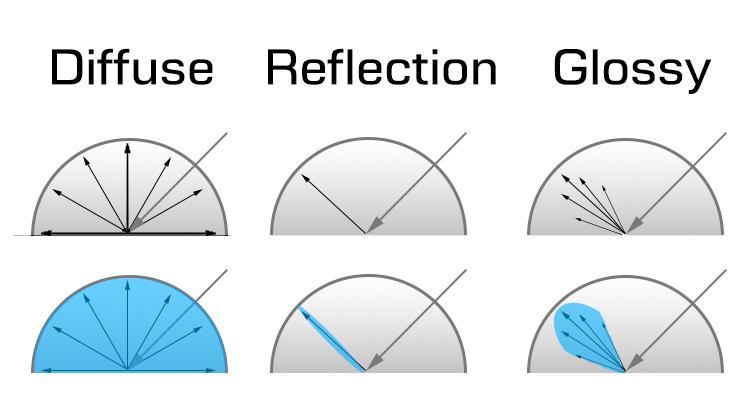
Figure 9: Top is a comparison of the ray bounces for the material compared to the original hemisphere sample space. Bottom in blue depicts the actual hemispherical sample space associated with this type of material.

2.3 Multiple Importance Sampling

To get multiple interesting materials, these sample spaces can be superimposed and normalized in association with one another such that the overall pdf of the sample space still sums to the surface area of said space. That is, our value of 1 for the pdf in this case is the total surface area over which a sample can be chosen.

There are some other interesting materials such as microfacet materials in which the skewed hemisphere is also heavily imbalanced. This leads to interesting random specular highlights that given the right probabilities can even be turned into images [Figure 10].

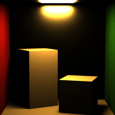
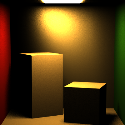
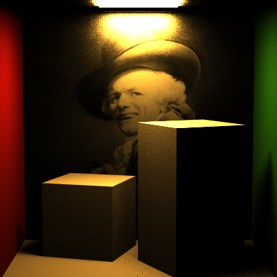
Figure 10: Left - microfacet background. Middle - microfacet background with increasing diffuse properties. Right - microfacet background with image-noise-based diffuse properties.

All scenes depicted so far have had one light, but if light is additive, there needs to be a way to proportionally incorporate multiple lights in a scene without blowing it out. Multiple Importance Sampling (MIS) does just this. Using a heuristic function usually on the exponential scale, it renormalizes the light field such that the combinations of the lights sums to the original value of 1 (i.e., [1, 1, 1] for white light) [Figure 11]. Note that if the lights are different colors or intensities, this heuristic becomes skewed based on the proportion of those intensities in relation to one another.

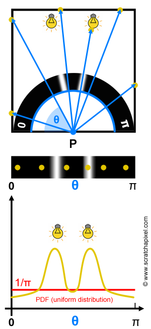
Figure 11: The normalization of the probability function for how each light’s intensity and color should be incorporated into final color values. Note that this image depicts the heuristic for two lights of the same intensity and color so the skewing is symmetric.

This effect can also be used to correct color values for sampling small versus large lights, which is one of the reasons why the MIS heuristic must be used. General Lighting is lighting found by doing probabilistic ray bounces without trying to hit the light specifically (i.e., just following the recursion direction). Direct Lighting has no recursion and is sampling the light from an intersection in the scene to see 1) if the light is in view and 2) what the color is at sampled probability location intersected on the light.

In [Figure 12] the main issues of General Lighting and Direct Lighting without MIS are highlighted. For General lighting, it is that for small light sizes, the surface area is too indistinguishable so the rougher surface further out is incredibly noisy. For Direct Lighting, it is that for large light sizes, the sampling of the light based on the probability of the intersection is too low leading to the speckled effect on the closer smoother surface. Using an exponential heuristic that proportions the pdf of the light and surface depending on which of those were used, the algorithm proceeds by only sampling one light per bounce. In doing so, it assumes that the heuristic evens out the different lights’ contributions based on the large number of bounces and samples per pixel. Note how the third image is nicely rendered for all light types and all surfaces.

A common heuristic used is the Balance Heuristic as follows. Note that the variance for one ray calculation is used to actually determine the color output value using this heuristic since the code uses a recursive aspect to accumulate the color value:

w_i(x) = \frac{n_i \cdot p_i(x)}{\sum_k n_k \cdot p_k(x)}

f = \sum_{i=1}^{n} \sum_{j=1}^{n_i} \frac{f(X_{i,j})}{\sum_{k}^{n} n_k \cdot \text{pdf}_k(x)}

For 1 ray: f = \frac{f(\omega_i)}{n_{L_i} \cdot \text{pdf}_{L_i} + n_{L_o} \cdot \text{pdf}_{L_o}} + \frac{f(L_o)}{n_{L_i} \cdot \text{pdf}_{L_i} + n_{L_o} \cdot \text{pdf}_{L_o}}

Code-wise, 1 ray converts to: \frac{nf \cdot f_{\text{pdf}}}{nf \cdot f_{\text{pdf}} + ng \cdot g_{\text{pdf}}}

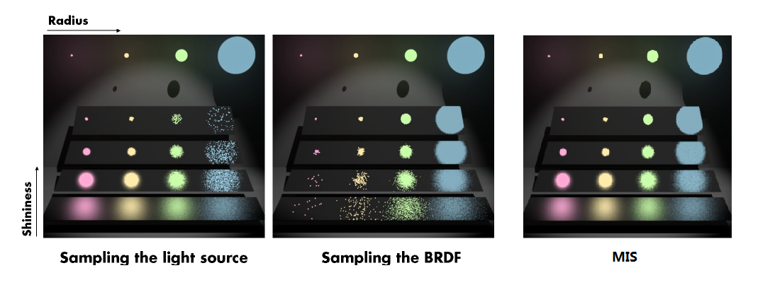
Figure 12: Three images of different rendering aspects at 100 spp depicting the lighting of increasingly sized lights on surfaces of differing roughnesses (purple to orange is smooth to rough). Note all these images have emissiveness (L_e) in their rendering code so the sphere lights themselves show up. Left - Direct Lighting. Middle - General Material Lighting. Right - Multiple Importance Sampling.

2.4 Entropy Based Adaptive Sampling

So far, in all the rendered images, each pixel has been rendered in the same fashion. That is, each pixel, regardless of how noisy or not its output will be, is rendered with the same number of spp. This is incredibly costly in terms of runtime and memory. Especially in places where the material is heavily uniform and diffuse or not even intersecting anything in the scene. One way to reduce this cost is through entropy-based adaptive sampling. That is, instead of sampling each pixel with the same number of samples as the pixel next to it, first do a pass to determine the materials to be directly sampled with a reduced count. Then, if necessary, continue adding more sample checks to the pixel until it reaches a convergence level below the error mark.

This explanation will be using Renyi’s Entropy, which is a more precise extrapolation of Shannon’s entropy.

Shannon’s Entropy: H_k = -\sum_{l=1}^{n} p_l \cdot \log_2(p_l)

Pixel Quality for each Spectral Channel: Q_k = \frac{H_k}{\max H_k}

Average spectral value for all Pixel rays for a specific channel: \bar{s}_k = \frac{1}{n} \sum_{l=1}^{n} s_l

Pixel Quality as a whole: Q = \frac{\sum_{k=1}^{n_s} w_k \cdot Q_k \cdot \bar{s}_k}{\sum_{k=1}^{n_s} w_k \cdot \bar{s}_k}

Now take into consideration Renyi’s Entropy: H_k^R = \frac{1}{1-q} \log_2 \left( \sum_{l=1}^{n} p_l^q \right)

To get our final formulas we use Renyi’s Entropy calculation to rewrite the Pixel Quality for each Spectral Channel, which in turn rewrites the Pixel Quality as a whole for each pixel.

Renyi’s Pixel Channel Quality: Q_k^R = \frac{H_k^R}{\log_2 n}

Pixel Quality as a whole using Renyi’s Entropy: Q = \frac{\sum_{k=1}^{n_s} w_k \cdot Q_k^R \cdot \bar{s}_k}{\sum_{k=1}^{n_s} w_k \cdot \bar{s}_k}

Comparing the results in [Figure 13], notice a distinct difference in noise of the result. Renyi ran much faster than Shannon by itself, and required much less memory to converge in the first place.

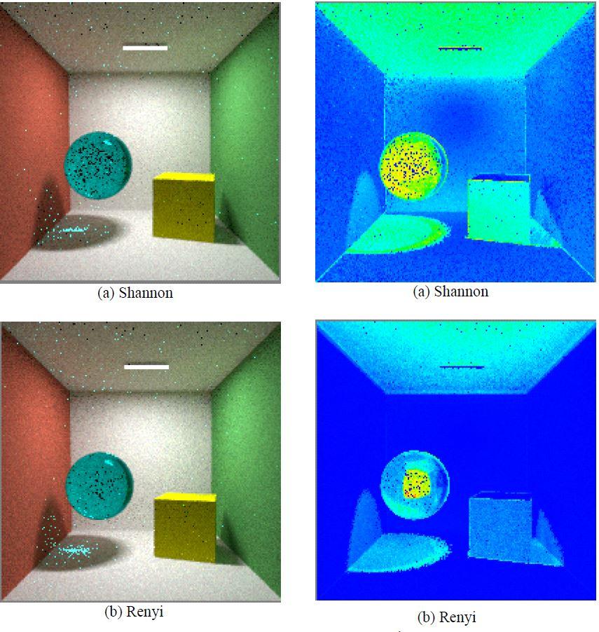
Figure 13: Color indicates the number of samples required for the specific pixel to converge. Note that there is much more solid blue in the Renyi second image indicating more pixels that required fewer samples in the first place to reach about the same output as the Shannon version. The bit of blue speckled noise in the rendered left versions of both Shannon and Renyi is due to the refractive sphere that has not been handled properly.

2.5 Photon Mapping

Another way to fake this convergence mentioned in the Entropy section is to use photon mapping. Albeit this heavily increases the memory required for the application; however, it runs much faster because it relies on the brain’s own obfuscation. Human eyes will believe blur much more easily than noise. Looking back at the previous images in this paper, it’s easy to notice their fake qualities. The variance in pixel colors in close proximity, the sometimes black pixels on an object, and other details the eyes pick up on that scream to the viewer, “this isn’t real.”

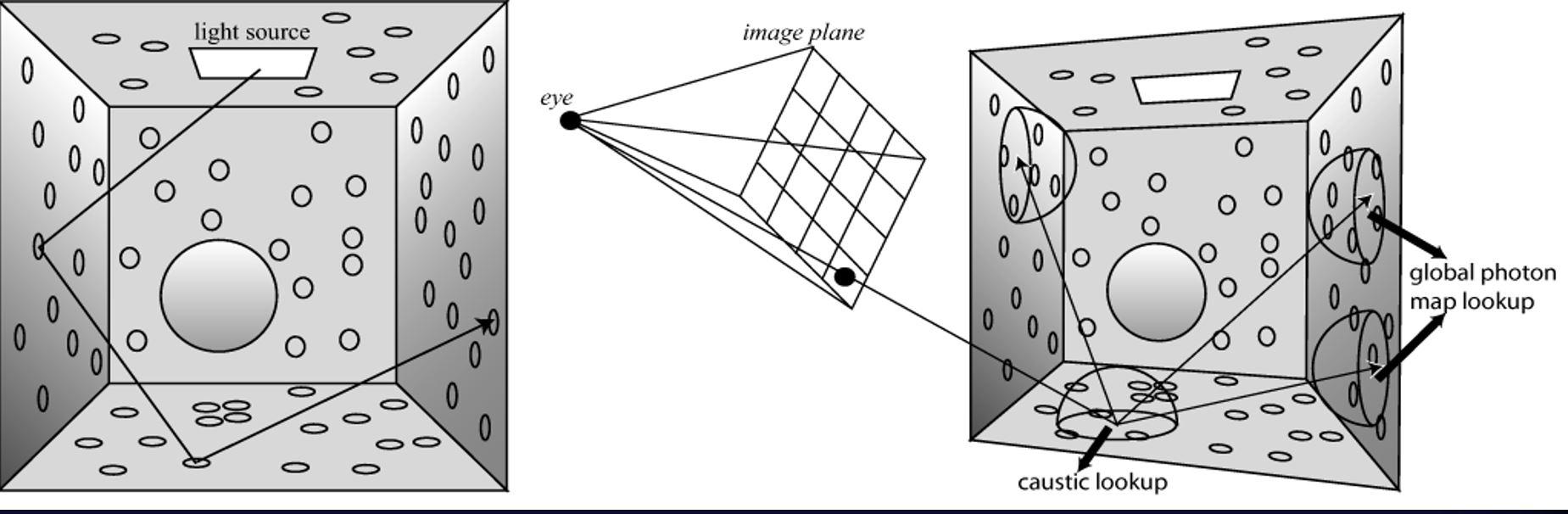
Figure 14: The two stages of Photon Mapping. Left - storing. Right - looking up what was stored and rendering based on those values.

Photon mapping involves two stages [Figure 14]: 1. Store photons in the scene based on the materials they hit. 2. When actually rendering, check the one intersection in the scene for possible directions; at those directions check the stored photon values within a particular distance on a surface. That is, actually follow how light would reach a surface, then blur it based on the averaging.

Considering PathTracing versus Photon Mapping, the latter does a pre-storing of all the ray bounce information that path tracing might need to recalculate at each intersection iteration; however, both technically do the same number of calculations. That is, Path tracing is to Photon Mapping as Recursion is to Dynamic Programming. They both technically do the same thing but one is more optimal than the other.

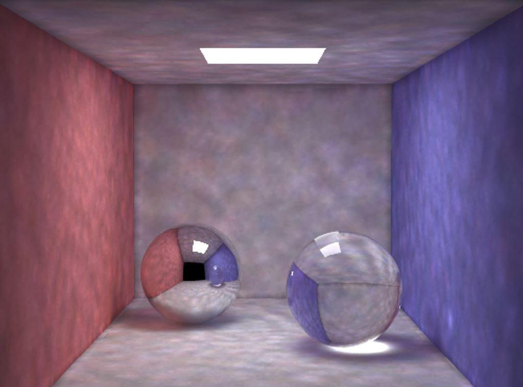
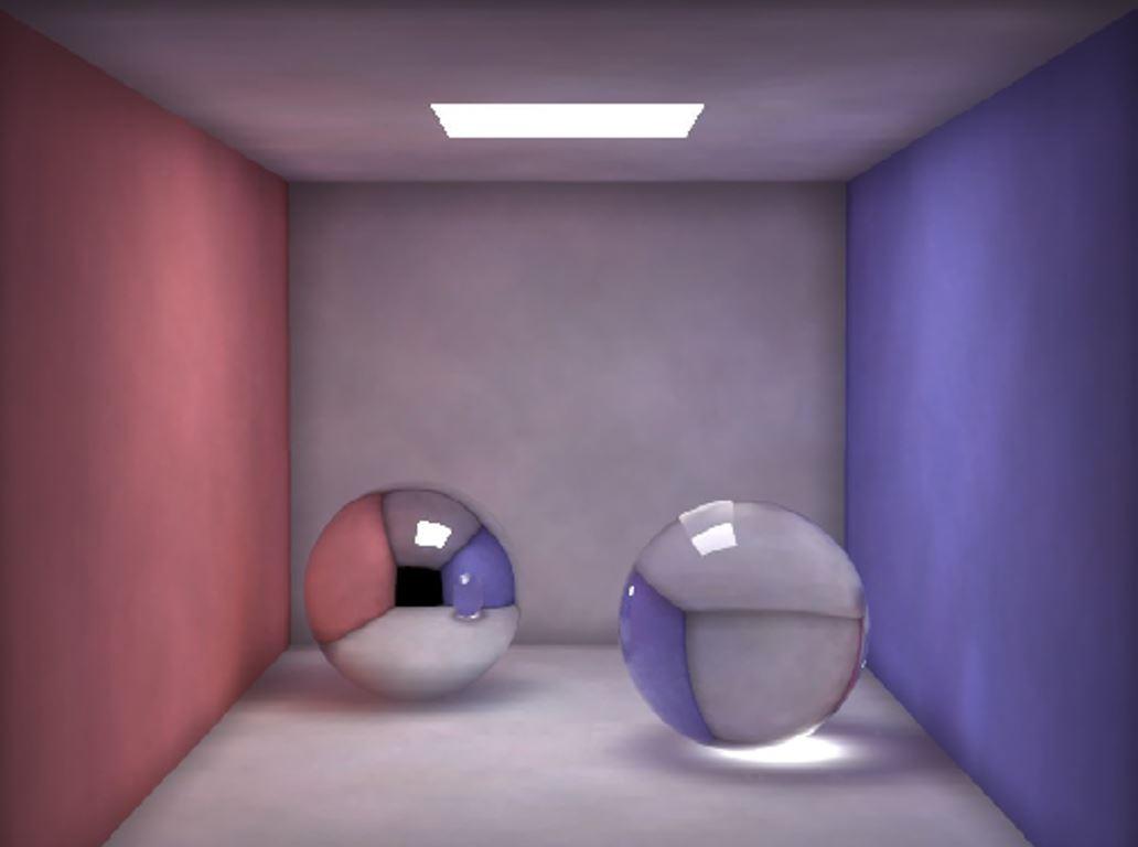
Figure 15: A comparison of photon mapping with ~1,000 photons in the scene versus ~100,000. Both are rendered at 3 spp which is still much lower compared to the usual 100 \times 100 spp required for general pathtracing to converge to the right image.

Part II: The Image Compression Problem

Introduction

As was mentioned in the introduction, our visual system gives us the ability to sense ~30 frames a second of color imagery, equating to about 1 Gigabyte/second of visual data. What’s even more impressive is that unlike a DVD, our eyes and minds are not only acquiring and storing this much data, but processing it for a multitude of tasks: from 3-D rendering to color processing, from segmentation to pattern recognition, from scene analysis and memory recall to image understanding and finally data archiving, all in real time.

Obviously we don’t remember everything that we see, but the fact that we are still able to reconstruct some important images/moments/events with nearly perfect clarity raises the question of how we possibly store all of this data. While our understanding of the brain is still quite limited, current estimates place the Brain’s processing and storage power between 1 terabyte to 2.5 petabytes. This, however, is only equivalent to about 2 months worth of full sensory data. Clearly, our brains must be imposing some sort of compression system to allow us to store more than 2 months of visual data in our memory. This is also evident from a perceptual level since we can often look at compressed images (think of the JPEGs stored automatically by your camera) and see close to no difference from the full image (a phenomenon called transparency).

Image compression is also highly relevant to the tech industry, for it is estimated that close to 80% of global bandwidth is taken up by video traffic (15% of which is Netflix alone). Any improvements that can be made to improve the transmission of this data means faster downloads and happier customers.

Here we will explore the mathematics and applications of one of the most useful computational tools for image compression: the wavelet. Although purely a mathematical object, wavelets are hypothesized to play a role in the human visual system as well.

Wavelets

Wavelets are a class of functions that are very efficient in discriminating actual data from noise data, hence their application in signal/image processing as filters. Unlike other signal processing tools such as Fourier transforms, which only use a linear combination of sines and cosines to approximate a function, wavelet transforms use an infinite set of functions of different scales and at different locations to perform the same task.

This is important because while mathematically one orthonormal basis is as good as another, it turns out that in signal processing there can be significant practical differences between orthonormal bases in representing particular classes of signals. For instance, there can be differences between the distribution of coefficient amplitudes in representing a given signal in one basis versus another, leading to representations that are more or less susceptible to compression.

A family of wavelets is composed of an infinite set of functions generated by rescaling and translating the scaling function, also known as the Father wavelet (\phi) and the wavelet function itself, which is also known as the Mother wavelet (\psi). The rescaled and translated functions are called son wavelets and daughter wavelets, respectively. While these families are infinite, we choose just a small subset to form our orthonormal basis.

Those familiar with the usefulness of the Fourier transform in other realms of signal processing may wonder why the same technique is not applied here. In truth, the real strength of Fourier-based methods is that oscillations—waves—are ubiquitous in nature. All electromagnetic and many other physical phenomena are associated with waves, which satisfy assumptions of stationarity. This stationarity means that the waves do not have local statistics (trends in different parts of the data) and can be easily approximated to the second degree. Naturally, waves are also important in vision, for light is a wave. But visual information doesn’t adhere to this stationarity. Instead, the content of natural images is typically that of variously textured objects, often with sharp boundaries, as we saw in the previous section on rendering. The objects themselves, and their texture, therefore constitute important structures that are often present at different “scales.” Much of the structure occurs at fine scales, and is of low “amplitude” or contrast, while key structures often occur at mid to large scales with higher contrast.

Thus we note that a basis more suitable for image compression should represent information at a variety of scales, such that it can represent local contrast changes as well as larger scale structures. Keep this in mind as we continue our discussion on wavelets.

Indeed, the discovery and increased study of wavelets grew quite directly from the shortfalls of the Fourier transform. In order to analyze non-stationary signals that the Fourier transform struggled with, scientists created the modification of the Fourier transform called the Short Time Fourier Transform (STFT) in 1946. The STFT looked to improve its time localization by segmenting the signal into windows and computing the classical transform in each window. In the late 1970’s, J. Morlet faced the problem of analyzing signals which had high frequency components with short time spans and low frequency components with short time spans—kryptonite for the STFT. He then came up with the idea of using different window functions for analyzing different frequency bands, with each window generated by a dilation or compression of a prototype Gaussian. Due to what he called the “small and oscillatory” nature of these window functions, Morlet named his basis functions as wavelets of constant shape. Yves Meyer and J.O. Stromberg (re-)discovered orthonormal wavelet basis functions in the mid 1980’s, but the field did not truly flourish until Daubechies and Stephane Mallat (a graduate student at UPenn!) developed the transform for discrete signal analysis. Mallat’s Ph.D. thesis on multiresolution analysis in 1988 pushed the idea of decomposing a discrete signal into dyadic frequency bands by a series of different high pass and low pass filters to compute its discrete wavelet. This idea, along with the growing technological transformation, helped spur great interest in the field and led to notable advancements in signal processing.

Here we limit our scope to one of the first orthonormal bases discovered, and use this wavelet to explore how the wavelet transform is used in image compression.

The Haar Wavelet

The Haar Wavelet was invented all the way back in 1909 by the German mathematician Alfred Haar, long before the work of the abovementioned pioneers. Although Haar wavelets are the first and simplest orthonormal wavelets, they are of little practical use because of their poor frequency localization. Still, they serve as a useful pedagogical example.

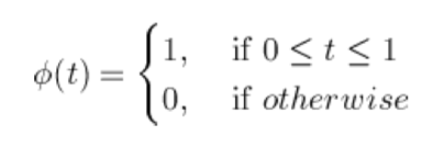
The Haar wavelet is defined as follows:

Father Wavelet:

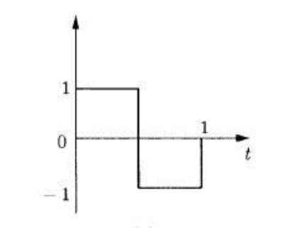
Mother Wavelet:

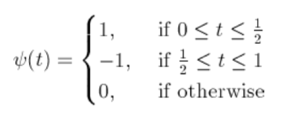
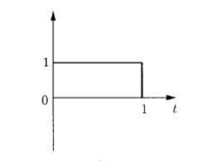
With the father wavelet on the left and the mother wavelet on the right. In addition, the son wavelets and the daughter wavelets are rescaled and translated according to parameters n and k as follows:

Note that while a change of parameter n allows one to look at the function or signal at different scales, a change in parameter k allows one to localize the function at a desired position. This means that each daughter and son wavelet is an individual function that is a member of a wavelet family. As a whole, a family of wavelets allows us to analyze both the larger trends and the details of a signal, which we will see come in handy as we try to decompose an image. Also observe that intuitively, the father wavelet takes the sum of the points in its range and then takes their average in order to normalize the function, while the mother wavelet finds the difference of adjacent regions. It’s easy to see that applying these two functions on a data set retains information since the values of two numbers can be completely determined by their average and their difference.

Demonstration

We will now explore how Haar wavelets can compress an image using a familiar photograph as an example. We will simplify our calculations by squishing the image into a 256 \times 256 grayscale image, which we will denote f.

We begin by using the Haar transform over j = 1, \ldots, \log_2(256) scales, computing the coarse and fine scale coefficients (c_j, H_j, V_j, D_j) where j \in \{1, \ldots, 8\} and H, V, and D designate the horizontal, vertical, and diagonal coefficients, respectively, at each level. While these coefficients represent the image regardless of their organization, the natural representation of an image as a two-dimensional matrix, along with the fact that computing the coefficients at a larger scale is equivalent to recursively doing the same computation on the previous result, allows for a visually appealing representation. We note that this form is achievable due to the nice property of Haar wavelets being averages and differences at different scales. Computations with other wavelets are much less intuitive.

We initialize our algorithm by letting c_0 = f and then define each subsequent scale iteratively as follows.

For the vertical transformation, we apply the one-dimensional Haar transform on every column of the previous scale. That is to say, for all j \in \{1, \ldots, \log_2(256)\} and k \in \{1, \ldots, 2^{8-j}\} we calculate:

We then use the same one-dimensional transform horizontally in order to obtain our coefficients at scale j (i.e., the next upper left quadrant):

Here’s what our matrix looks like after just the vertical transform and then after a full iteration:

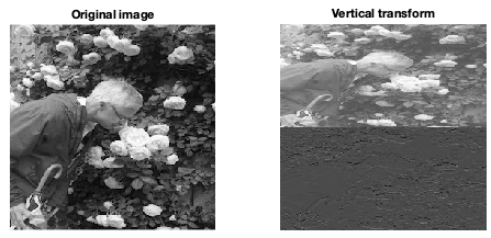
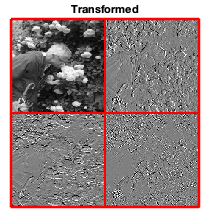
After \log_2(256) - 1 = 7 more iterations of this algorithm, we obtain all of our coefficients, resulting in a fractal-like form with the single average of all averages in the top left.

But what’s the point of all of this, you may ask, since we are still left with a 256 \times 256 matrix of pixel data, which is exactly what we started with. The answer is more apparent when you take a closer look at the matrix data, and notice that many of the entries are now very close to being zero. This is important because we can encode a sparse matrix (one with many zero entries) very efficiently using entropy encoding techniques. Once encoded, the data can then be sent over the network (or stored in synapses) and recapitulated (accessed) on the other end with knowledge of the encoding scheme.

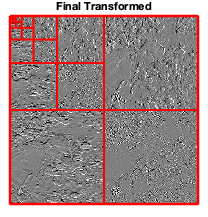
Up to this point, our image compression has been lossless, which is to say that we have lost no information so far in this process and thus if we were to take the inverse transform of our final transformed matrix, we would be handed back the exact same image that we started with. This is useful if we care about the finest of details, but as we will see with our image, some data loss is barely perceivable. The upside of changing to a lossy scheme is that it will allow us to encode our image even more efficiently since our information loss comes in the form of ‘zeroing’ values that are close to zero. There are three main ways that this is done:

1. Hard threshold: Substituting all coefficients whose absolute value is below the selected tolerance with a zero.
2. Soft threshold: Carrying out a hard threshold but also shifting all of the other entries by the tolerance.
3. Quantization: Zeroing the smallest p percent of entries (most common in practice).

For this example we thresholded our coefficients using a cutoff value of 0.1 (grayscale values range from 0 to 1), resulting in the thresholded matrix below.

Even in this representation we can see that a fair bit of the detail in the differences was lost due to the thresholding. Numerically, the impact was even larger, as the number of zero entries grew from 576 in the original coefficient matrix to 53,950 in the thresholded matrix out of 256 \times 256 = 65,536 entries.

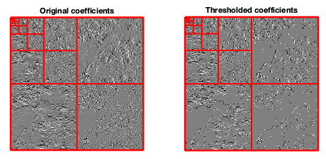
To see the impact of this thresholding on the final image we first need to define our inverse transform function. We can do so simply by starting now from c_8 and then computing c_0 from c_1, H_1, V_1, and D_1 by first computing the inverted horizontal transform for all appropriate indices:

And then using the inverted vertical transform to finally find c_0:

Our transformations allow us to iteratively reconstruct the image as we receive more and more of the coefficients. This is especially useful in industry, as websites will often load a blurry image first using the initial iterations of the inverse transform, and will improve the reconstruction as more data comes through the network.

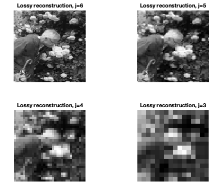
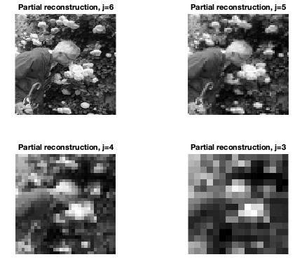
As you can see above there is almost no perceptual difference in the two reconstructions, despite the massive difference in sparsity (and thus compressibility).

Compression Protocols

In general, image compression is carried out using the following workflow: first the image is broken down into color components, often in a color space other than RGB in order to allow for better floating point rounding. After color segmentation, the image is split into tiles, or rectangular regions of the image that are transformed and encoded separately. These tiles are then each transformed using the Discrete Wavelet Transform, which uses filter banks in order to run in O(n) time (similar to the Fast Fourier Transform). The wavelet of choice for many leading wavelet compression protocols is the Cohen-Daubechies-Feauveau wavelet, which has favorable support properties. Once transformed, the tiles are thresholded using the quantization method and then encoded using a variety of different techniques.

As an aside, our estimates of brain storage capacity are very rough, and come directly from the following back-of-the-envelope calculation: The brain contains about 100 billion neurons; each of these neurons is capable of making around 1,000 connections through its synapses—which do most of the work of data storage; multiplying each of these 100 billion neurons by 1,000 connections gives you 100 trillion data points, or about 100 terabytes of information.

Conclusion

Thus we have determined a few different ways to answer our questions. In terms of simulating our visual environment, we can replicate our surroundings using the Light Transport Equation, layerings of sampling techniques, and different bouncing techniques for tracing the light in the first place. Additional techniques such as Multiple Importance Sampling, Renyi-based Adaptive Sampling, Path tracing, and Photon Mapping also help improve these simulations in different contexts. In terms of storing this visual data, we’ve seen that wavelets are especially useful for representing image data with sparse matrices. These wavelets are scaled and translated across the sample in order to decompose an image into coefficients that are efficiently encoded using entropic techniques. Together, these strategies allow us to simulate fantastic worlds such as Westeros, and then stream such worlds to millions of viewers.